LLM pre-training and scaling laws

Pre-training Large Language Models

Source: DeepLearning.AI - Learn the fundamentals of generative AI for real-world applications

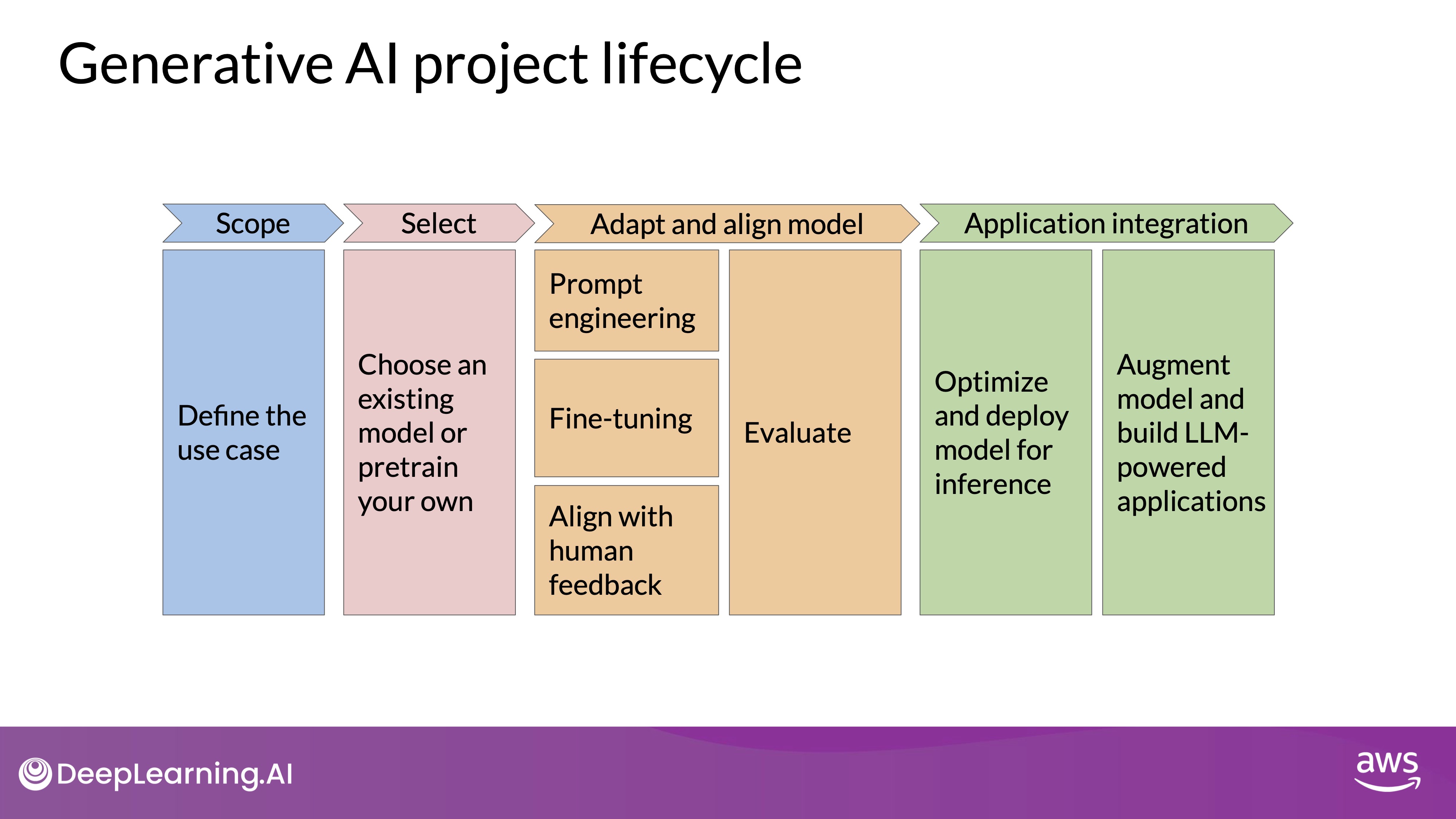
• Project Lifecycle: The development of a generative AI application involves several steps before launch. After scoping out the use case, selecting an appropriate model is crucial.
• Model Selection:
  • Choose between using an existing model or training a new one from scratch.
  • Generally, starting with an existing foundation model is recommended.

Existing Models and Model Hubs

Source: Hugging face: google/flan-t5-large

• Model Hubs: Platforms like Hugging Face and PyTorch offer curated hubs with many open-source models.
• Model Cards: These provide details such as best use cases, training methods, and known limitations, aiding in selecting the right model. For more details, check Hugging face: What are Model Cards?

Understanding Pre-training

TL;DR

• Model Architectures:
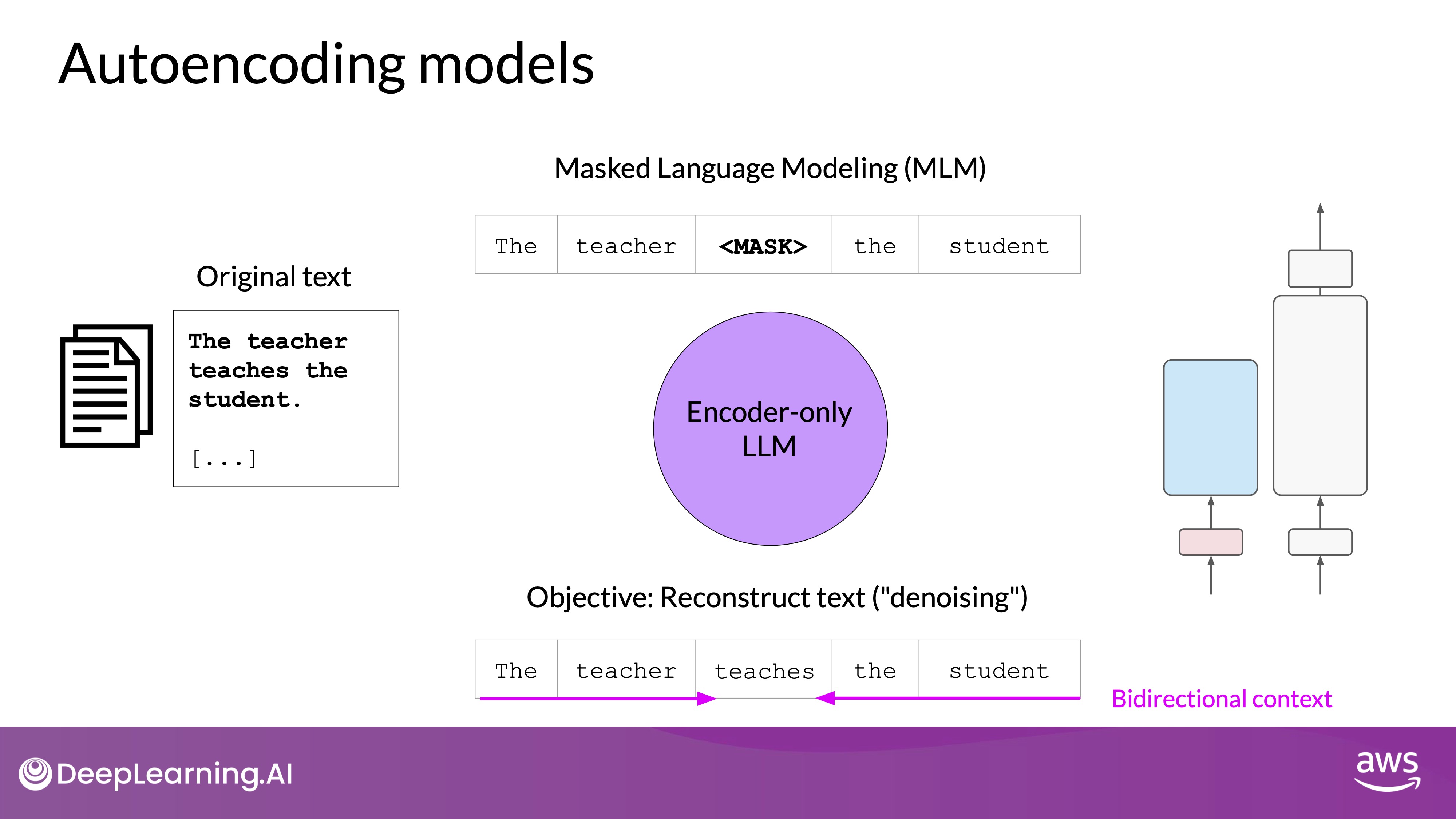
  • Autoencoding Models: Encoder-only, masked language modeling, suited for classification tasks.
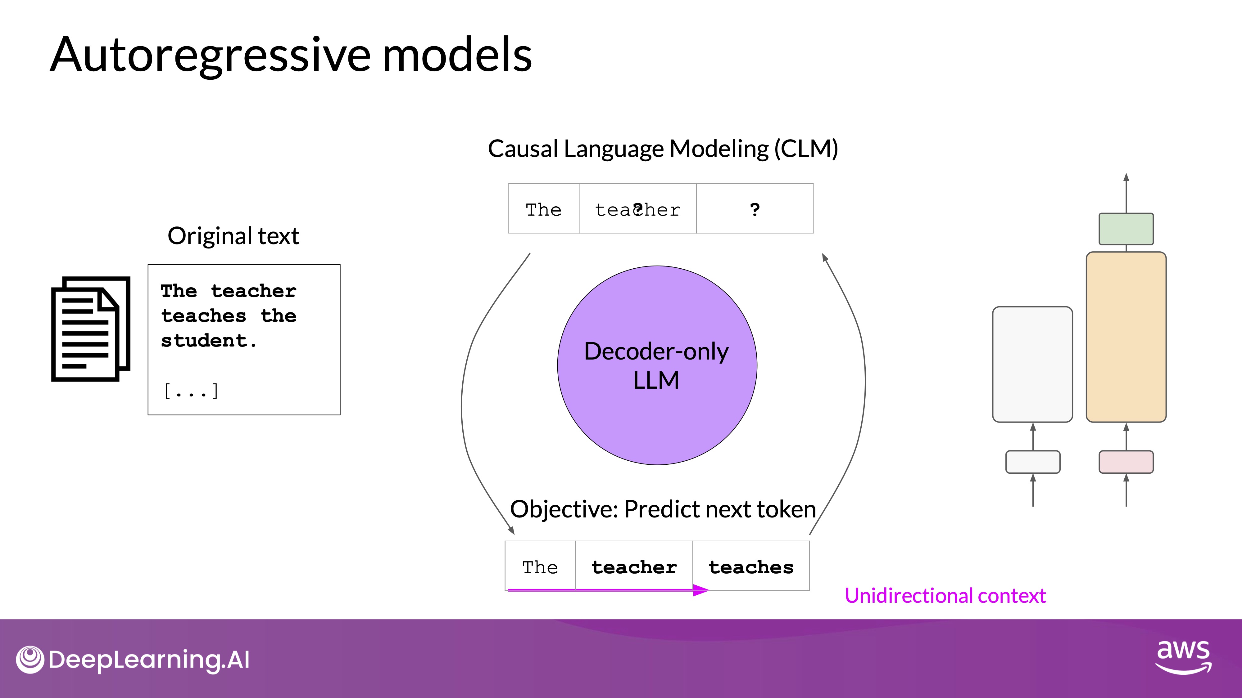
  • Autoregressive Models: Decoder-only, causal language modeling, suited for text generation.
  • Sequence-to-Sequence Models: Encoder-decoder, various objectives, suited for complex tasks like translation and summarization.
• Choosing a Model: Select based on the task, with larger models often providing better performance.

• Pre-training Phase: The initial training phase for LLMs, involving learning from vast amounts of unstructured textual data.
  • Data Sources: When you scrape training data from public sites such as the Internet, you often need to process the data to increase quality, address bias, and remove other harmful content. As a result of this data quality curation, often only 1-3% of tokens are used for pre-training.
  • Self-Supervised Learning: The model learns patterns and structures in the language to minimize the training objective loss. All it has to do is to predict the next word. There is not labled data

Training Objectives

Encoder-Only Models(Autoencoding)

Source: Hugging face: google/flan-t5-large

• Training Objective: Masked Language Modeling(MLM) - Predicts masked tokens to reconstruct the original sentence.
• Bidirectional Context: Understands the full context of a token and not just of the words that come before.
• Use Cases:
  • Encoder-only models are ideally suited to task that benefit from this bi-directional contexts.
  • Sentence classification (e.g., sentiment analysis), token-level tasks (e.g., named entity recognition).
• Examples: BERT, RoBERTa.

Decoder-Only Models (Autoregressive)

Source: Hugging face: google/flan-t5-large

• Training Objective: Causal Language Modeling - Predicts the next token based on previous sequence of tokens. Predicting the next token is sometimes called full language modeling by researchers.
• Unidirectional Context: Can only see preceding tokens, not subsequent ones. The model has no knowledge of the end of the sentence.
• Use Cases: Text generation, strong zero-shot inference.
• Examples: GPT, BLOOM.

Sequence-to-Sequence Models (Encoder-Decoder)

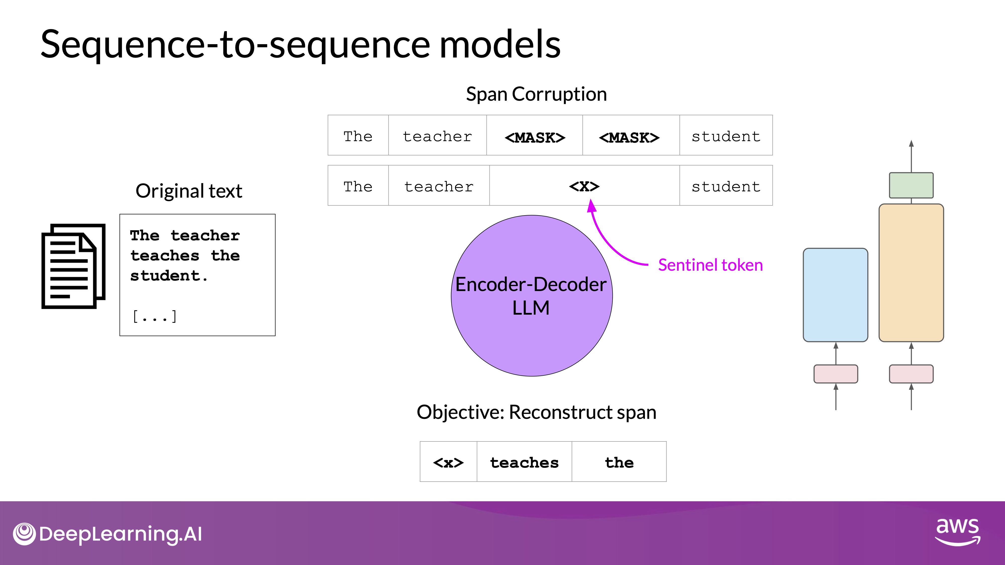
Source: Hugging face: google/flan-t5-large

• Training Objective:
  • The exact details of the pre-training objective vary from model to model.
  • T5 uses span corruption which masks random sequences of input tokens. Those mass sequences are then replaced with a unique Sentinel token, shown here as x. Sentinel tokens are special tokens added to the vocabulary, but do not correspond to any actual word from the input text. The decoder is then tasked with reconstructing the mask token sequences auto-regressively.
  • The output is the Sentinel token followed by the predicted tokens. <x> teaches the
• Bidirectional and Unidirectional Contexts: Uses both encoder and decoder parts.
• Use Cases: Translation, summarization, question-answering.
• Examples: T5, BART.

Model Size and Capability

• Larger Models: Generally more capable and perform tasks better without additional in-context learning or further training.
• Trend: Increased model size correlates with improved performance, driving the development of larger models.
• Challenges: Training large models is difficult and expensive, raising questions about the feasibility of continuously increasing model size.

---

Automodeforseq2seqLM

To give you an example, before transformers came along, we had to write a lot of this code ourselves. Depending on the type of model, there's now many different language models and some of them do things very differently than some of the other models. There was a lot of bespoke ad hoc libraries out there that were all trying to do similar things. Then Hugging Face came along and really has a very well optimized implementation of all of these.

What is a good model? Now some of you might be asking, well, this seems like cheating because we're actually giving it one answer and then asking it. It's not really cheating. It's more of you're helping the model help itself. Now in future lessons and in future labs, we will actually fine tune the model where we can go back to the zero-shot inference, which is what you would normally think of as a good language model.

Keep in mind, this is a very inexpensive way to try out these models and to even figure out which model should you fine tune. We chose Plan T5 because it works across a large number of tasks. But if you have no idea how a model is, if you just get it off of some model hub somewhere. These are the first step. Prompt engineering, zero-shot, one-shot, few shot is almost always the first step when you're trying to learn the language model that you've been handed and dataset. Also very datasets specific as well, and task-specific.

Here we see a case where the few-shot didn't do much better than the one shot. This is something that you want to pay attention to because in practice, people often try to just keep adding more and more shots, five shots, six shots. Typically, in my experience, above five or six shots, so full prompt and then completions, you really don't gain much after that. Either the model can do it or it can't do it and going about five or six.

Computational challenges of training LLMs

TL;DR

• Quantization: Key technique to reduce memory footprint by lowering the precision of model parameters, with FP16 and BFLOAT16 being popular choices.
• Memory Management: Critical for training large models, involving techniques like quantization and distributed computing.
• Future Challenges: Training increasingly larger models presents significant computational and financial challenges, highlighting the need for innovative solutions in AI research and development.

Memory Constraints

• Out-of-Memory Issues: Training or even loading large language models on Nvidia GPUs often leads to memory errors.
• CUDA: Libraries like PyTorch and TensorFlow use CUDA to optimize performance on Nvidia GPUs, but large models require significant memory.

Quantization

TL;DR - you can use quantization to reduce the memory usage(footprint) off the model during training.

• Memory Calculation
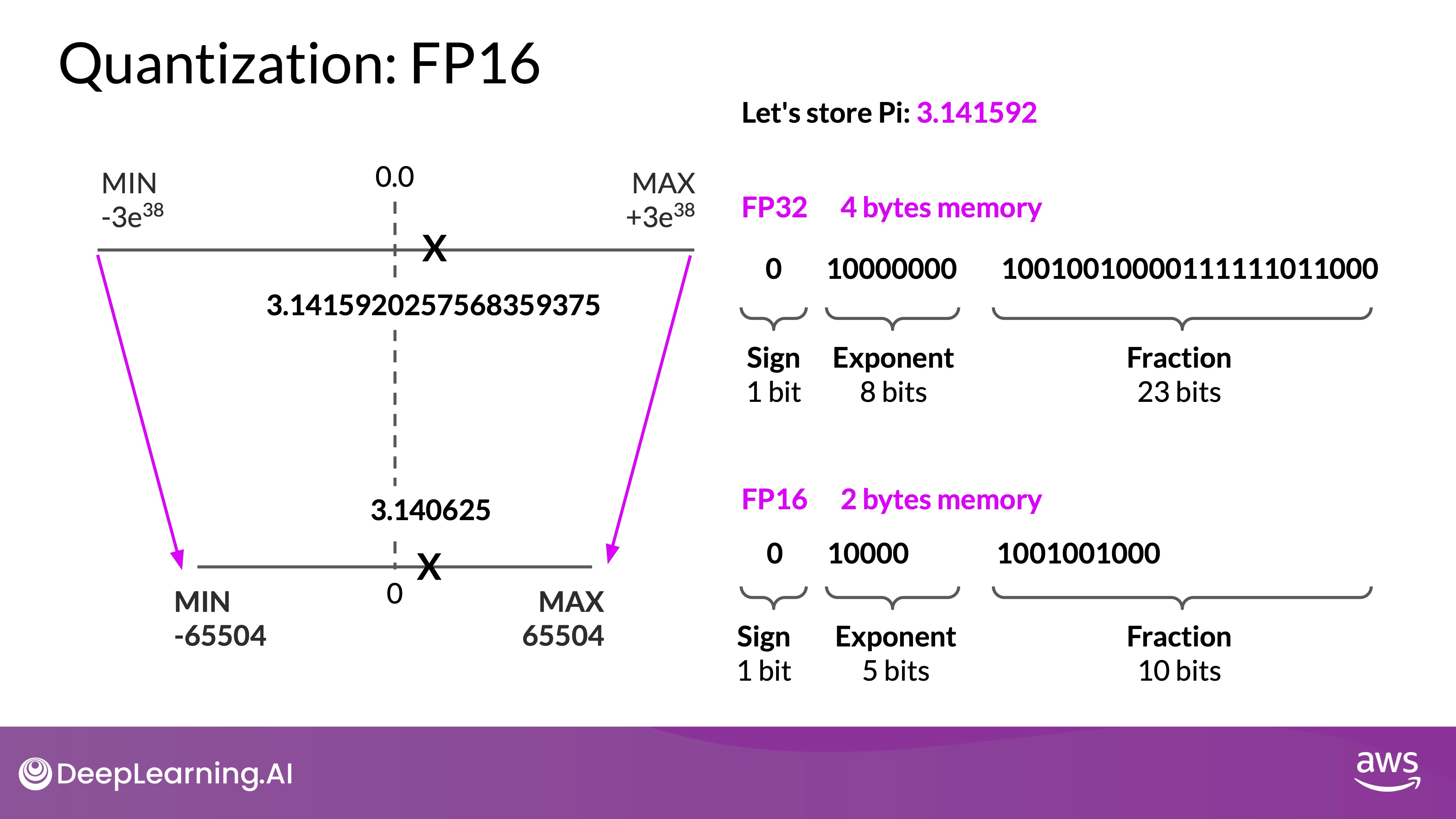
  • 32-bit Float Representation:
    • A single parameter in a model is typically a 32-bit float, taking up 4 bytes of memory.
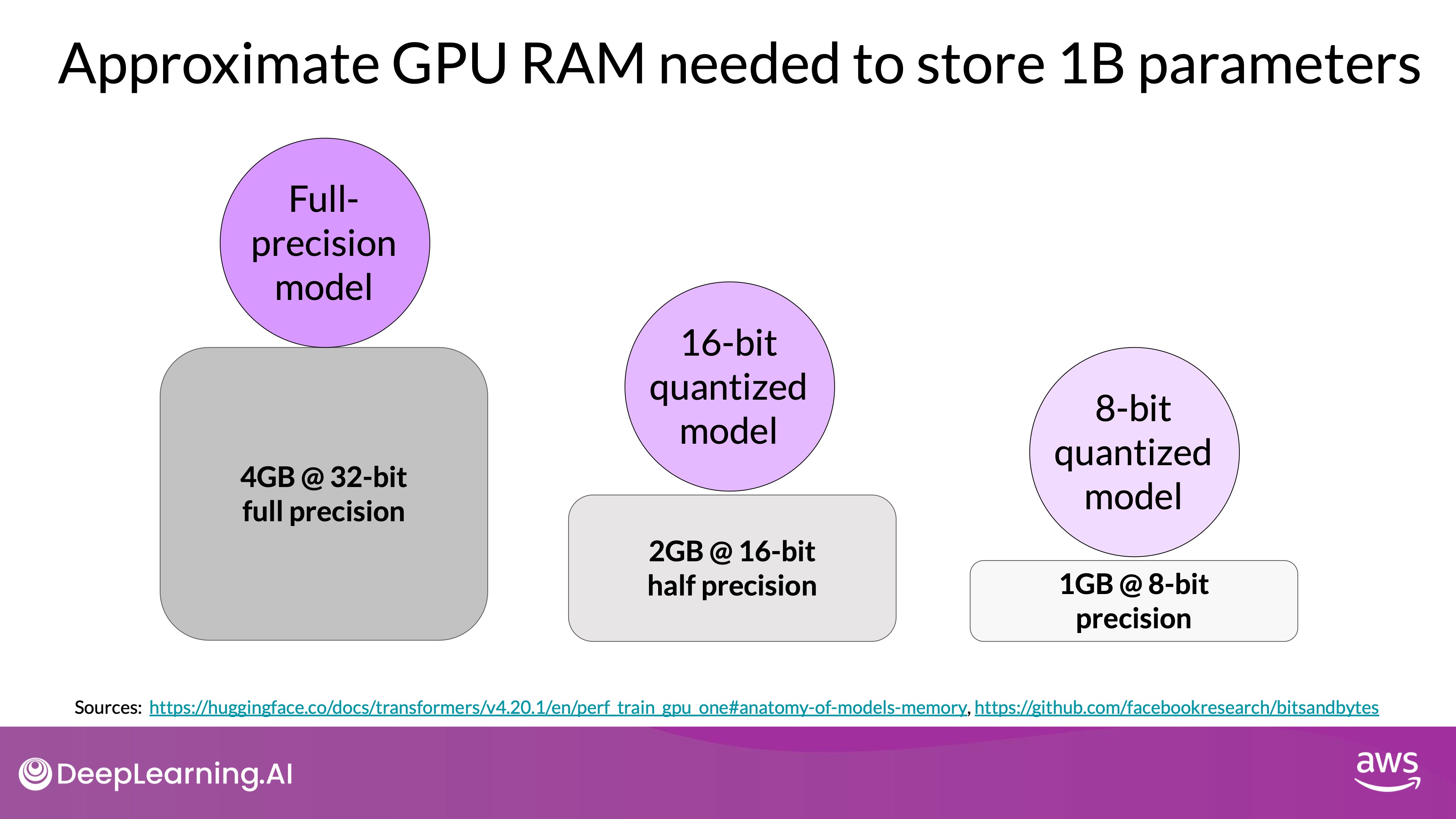
    • For one billion parameters, this requires 4 gigabytes of GPU RAM just to store the weights.
  • Training Overheads:
    • Additional memory is needed for optimizer states, gradients, activations, and temporary variables, often requiring 20 extra bytes per parameter.
    • Training a one billion parameter model at 32-bit full precision thus needs approximately 24 gigabytes of GPU RAM.
• Quantization:
  • Reduces memory by lowering the precision of model weights from 32-bit to 16-bit floats or 8-bit integers.
  • FP32 (32-bit full precision): Default representation.
  • FP16 or BFLOAT16 (16-bit half precision): Reduces memory usage by half, commonly used for training large models.
  • Source: DeepLearning.AI - Learn the fundamentals of generative AI for real-world applications
  • INT8 (8-bit integer): Reduces memory further but with significant precision loss.
• Precision and Range:
  • FP32: Can represent a wide range of values, but requires 4 bytes per value.
  • FP16: Uses less memory (2 bytes per value) with a smaller range and precision.
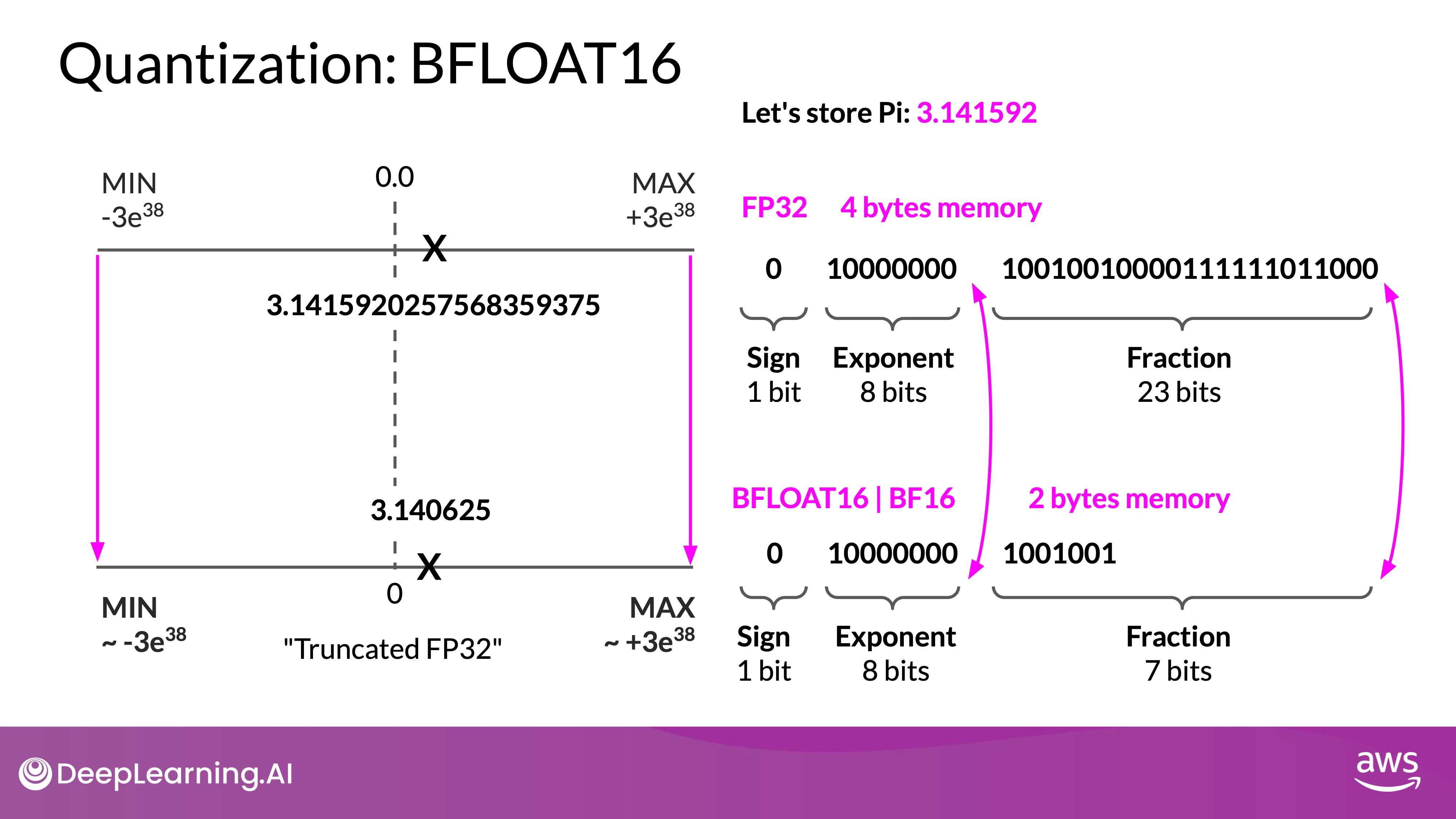
  • BFLOAT16:
    • Maintains FP32's dynamic range with 16-bit memory usage, offering a balance between precision and memory efficiency.
    • Many LLMs, including FLAN-T5, have been pre-trained with BFLOAT16. BFLOAT16 or BF16 is a hybrid between half precision FP16 and full precision FP32. BF16 significantly helps with training stability and is supported by newer GPU's such as NVIDIA's A100.
    • BFLOAT16 uses the full eight bits to represent the exponent, but truncates the fraction to just seven bits. This not only saves memory, but also increases model performance by speeding up calculations. The downside is that BF16 is not well suited for integer calculations, but these are relatively rare in deep learning.
    • BFLOAT16 has become a popular choice of precision in deep learning as it maintains the dynamic range of FP32, but reduces the memory footprint by half. Many LLMs, including FLAN-T5, have been pre-trained with BFOLAT16.
    • Source: DeepLearning.AI - Learn the fundamentals of generative AI for real-world applications

Takeaway

Remember that the goal of quantization is to reduce the memory required to store and train models by reducing the precision off the model weights. Quantization statistically projects the original 32-bit floating point numbers into lower precision spaces using scaling factors calculated based on the range of the original 32-bit floats. Modern deep learning frameworks and libraries support quantization aware training (QAT), which learns the quantization scaling factors during the training process.

Impact of Using Lower Precision Floating Point Representations

While using lower precision floating point representations does lead to some loss of information, this loss is often managed effectively through various techniques, making it a viable trade-off for the benefits of reduced memory and increased computational efficiency.

Even using Quantization doesn't mean it can reduce the model storage size

Source: DeepLearning.AI - Learn the fundamentals of generative AI for real-world applications

By applying quantization, you can reduce your memory consumption required to store the model parameters down to only two gigabyte using 16-bit half precision of 50% saving. Note that, you still have a model with one billion parameters. Quantization will give you the same degree of savings when it comes to training.

However, many models now have sizes in excess of 50 billion or even 100 billion parameters. Meaning you'd need up to 500 times more memory capacity to train them, tens of thousands of gigabytes. It becomes impossible to train them on a single GPU. Instead, you'll need to turn to distributed computing techniques while you train your model across multiple GPUs. Another reason why you won't pre-train your own model from scratch most of the time.

Efficient multi-GPU compute strategies

Large language models often exceed the memory capacity of a single GPU, necessitating the use of multiple GPUs to handle the extensive computational load. Even if a model fits on a single GPU, distributing the workload across multiple GPUs can significantly reduce training time by parallelizing computations.

Model Replication

Source: DeepLearning.AI - Learn the fundamentals of generative AI for real-world applications

Source: DeepLearning.AI - Learn the fundamentals of generative AI for real-world applications

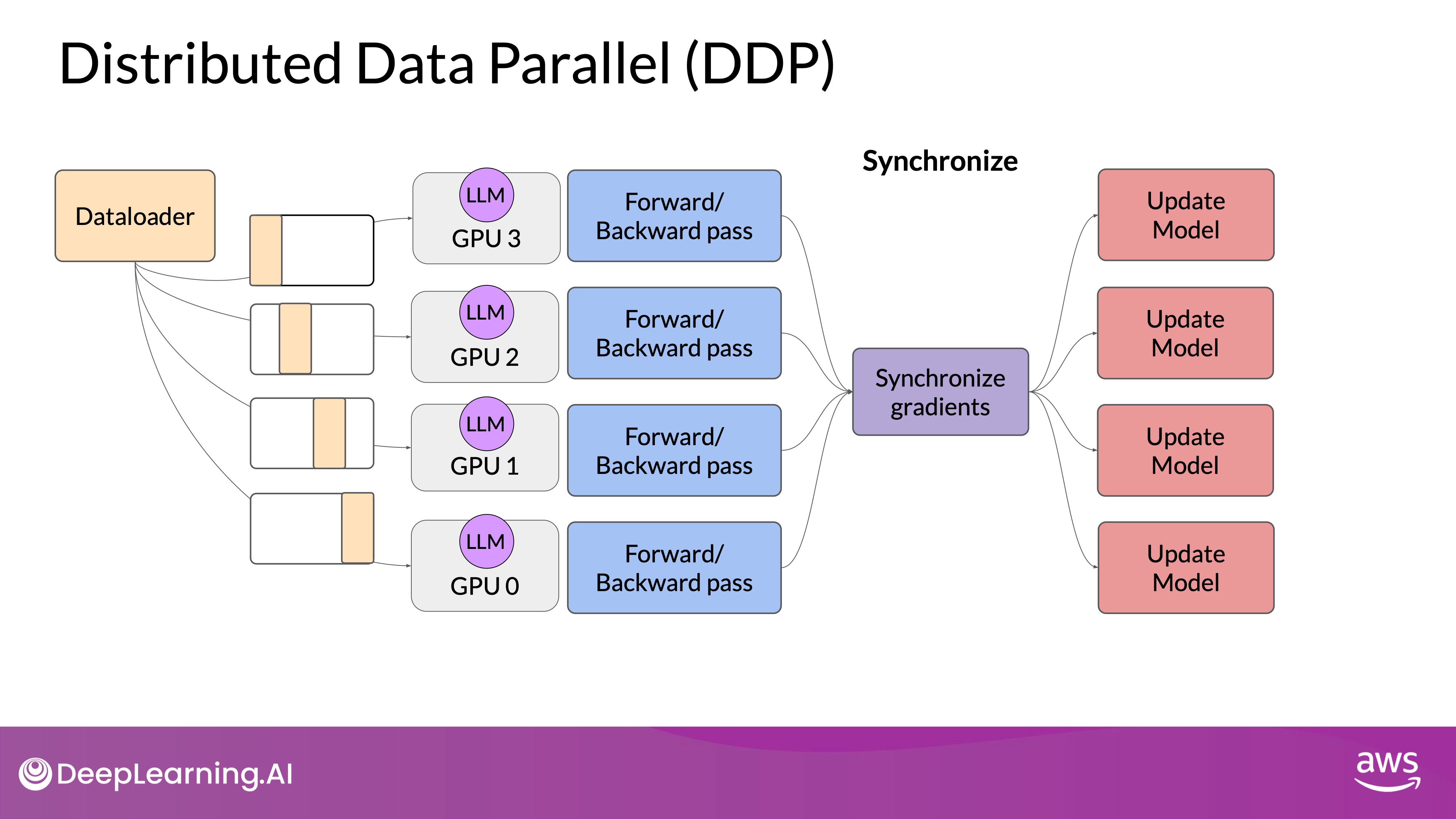
• Distributed Data-Parallel (DDP):
  • Implementation: DDP involves copying the model onto each GPU and dividing large datasets into batches that are processed in parallel by each GPU.
  • Synchronization: After processing the data, the results from each GPU are combined in a synchronization step, updating the model uniformly across all GPUs. This ensures that all copies of the model remain identical.
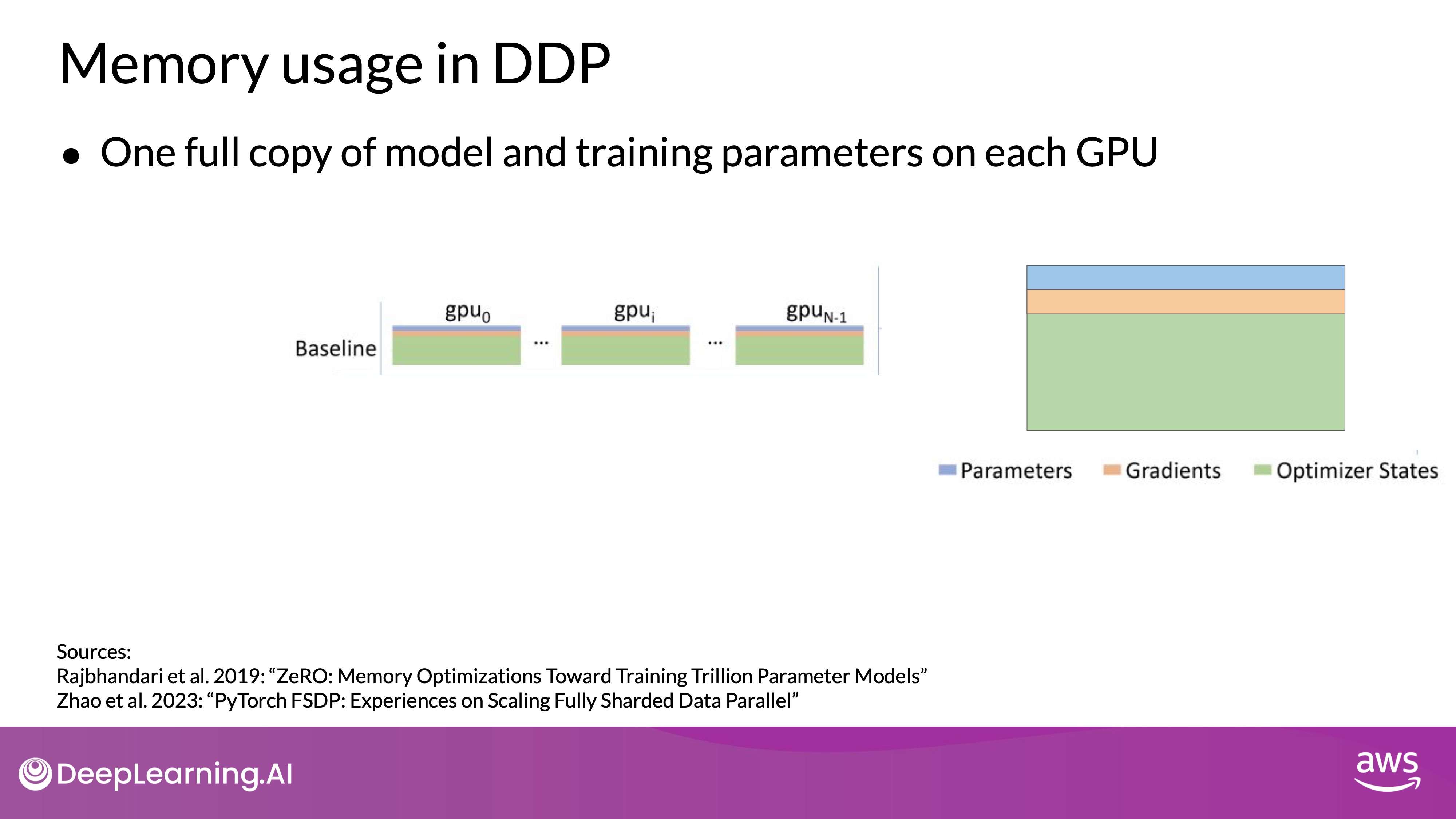
  • Memory Requirement: DDP requires that the model weights, gradients, and optimizer states fit within the memory of a single GPU, limiting its use for very large models.

You can't use DDP if you model can't fits into one single GPU

Note that DDP requires that your model weights and all of the additional parameters, gradients, and optimizer states that are needed for training, fit onto a single GPU. If your model is too big for this, you should look into another technique called modal sharding.

Model Sharding

Source: DeepLearning.AI - Learn the fundamentals of generative AI for real-world applications

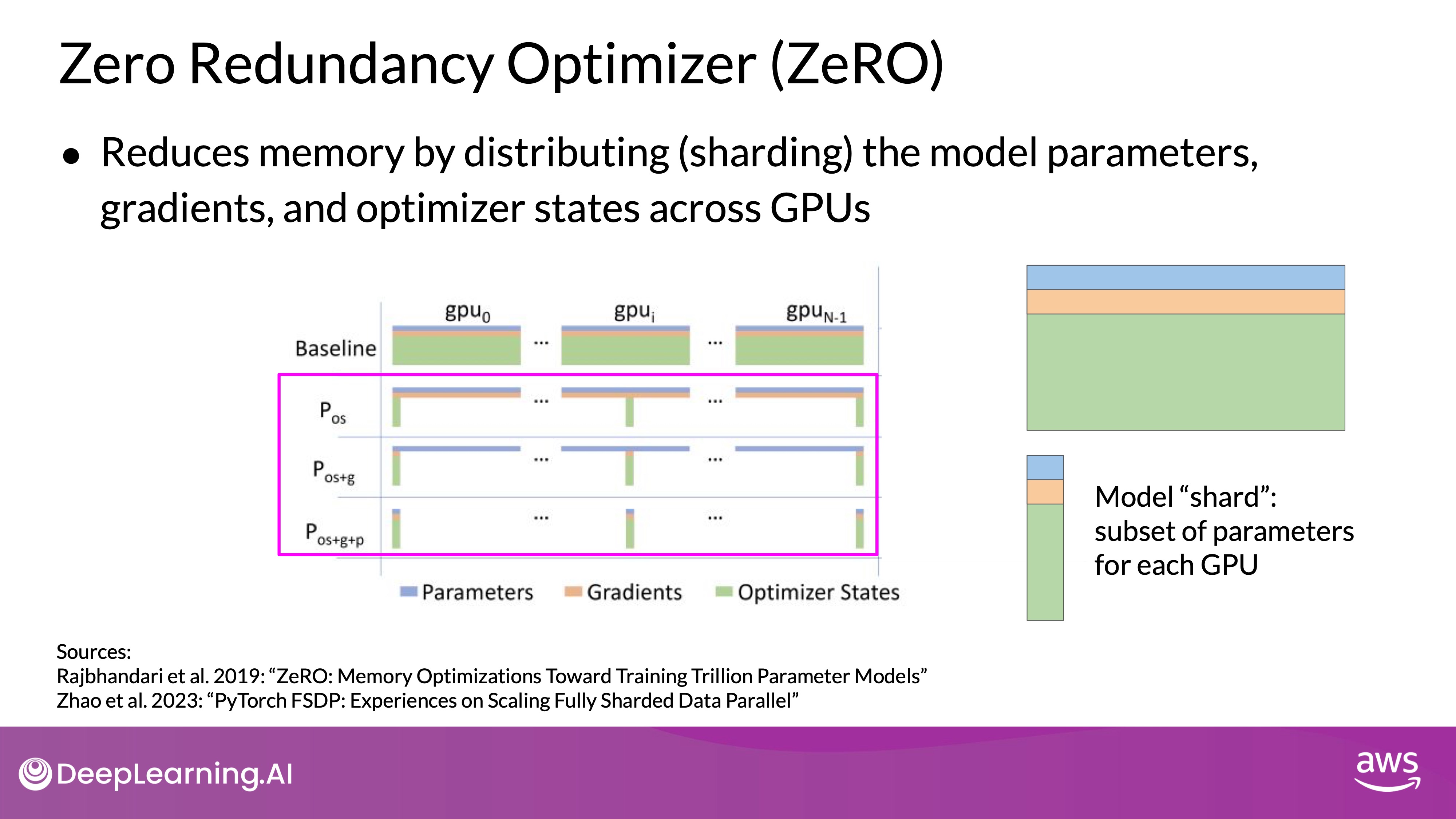
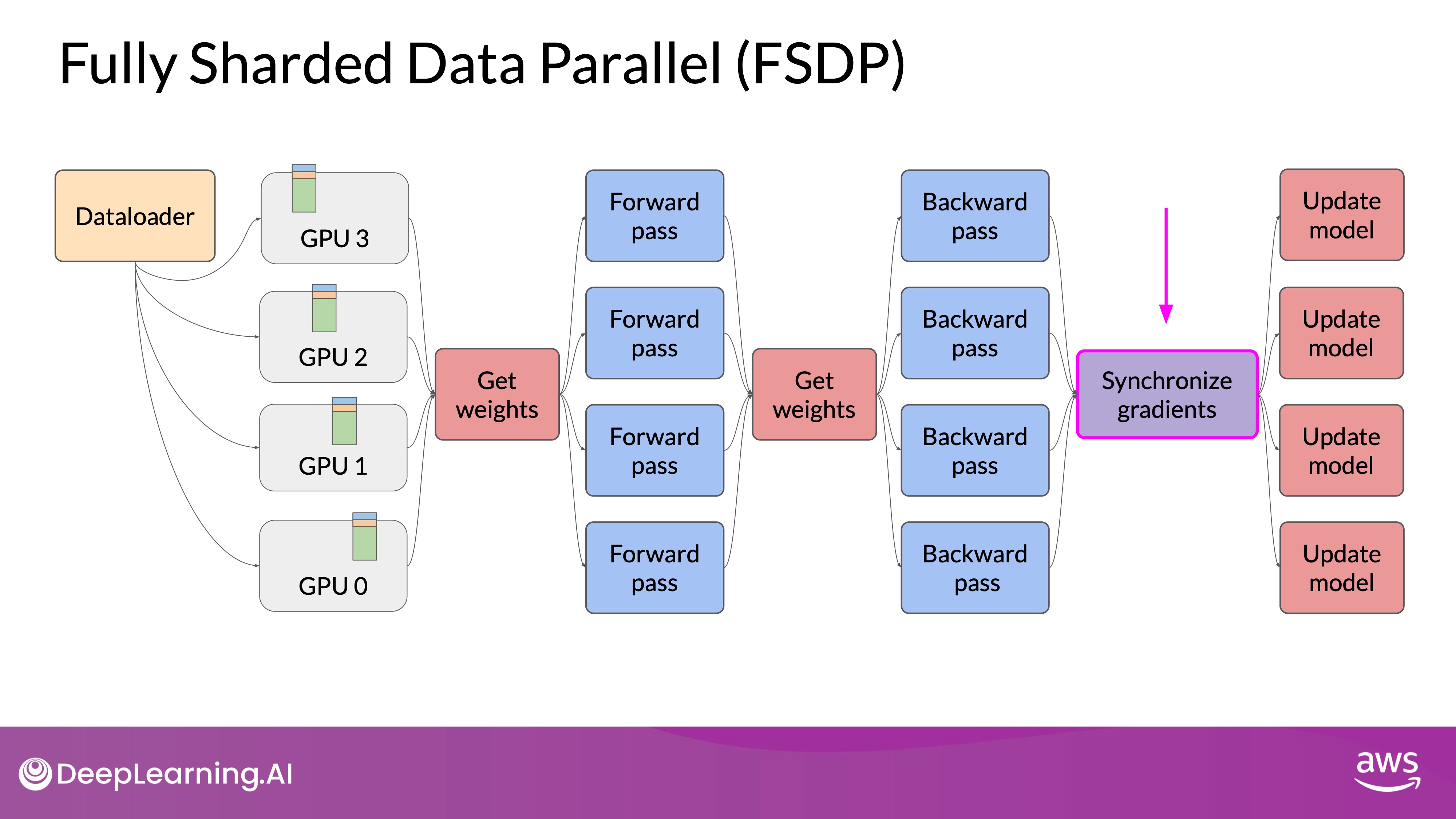
• Fully Sharded Data-Parallel (FSDP):
  • Concept: FSDP distributes (shards) the model parameters, gradients, and optimizer states across multiple GPUs instead of replicating them, based on the ZeRO (Zero Redundancy Optimizer) technique.
  • ZeRO Stages:
    • ZeRO Stage 1 ($P_{os}$): Shards only the optimizer states across GPUs, which can reduce memory usage by up to four times.
    • ZeRO Stage 2 ($P_{os+g}$): Shards gradients as well, potentially reducing memory usage by up to eight times.
    • ZeRO Stage 3 ($P_{os+g+p}$): Shards all model components, including parameters, gradients, and optimizer states, allowing memory reduction to scale linearly with the number of GPUs. For instance, sharding across 64 GPUs could reduce memory requirements by a factor of 64.

Source: DeepLearning.AI - Learn the fundamentals of generative AI for real-world applications

• Sharding Process:
  • Data Distribution: Data is distributed across GPUs, similar to DDP, but with the added advantage of sharding the model states.
  • On-Demand Data Collection: During the forward and backward passes, GPUs request the necessary data from each other, materializing the sharded data as needed for computations.
  • Release of Data: After operations, the non-local data is released back to its original shard, or retained if required for subsequent operations.
  • Synchronization: Following the backward pass, gradients are synchronized across GPUs, ensuring consistent updates.

Memory Utilization

• Reduction: FSDP can dramatically reduce the overall GPU memory utilization by efficiently distributing the memory load.
• Sharding Factor: The sharding factor controls the extent of sharding, ranging from full replication (similar to DDP) to full sharding across all available GPUs. Full sharding offers the highest memory savings but increases communication overhead.

Performance Comparison

• FSDP vs. DDP:
  • Small Models: For smaller models (e.g., up to 2.28 billion parameters), FSDP and DDP show similar performance.
  • Large Models: For larger models (e.g., 11.3 billion parameters), DDP may encounter out-of-memory errors, while FSDP can handle such models by effectively utilizing multiple GPUs. FSDP also achieves higher teraflops (trillions of floating-point operations per second) when models are reduced to 16-bit precision.
• Communication Overhead: As the number of GPUs increases, the volume of communication between GPUs grows, which can impact performance. This is particularly evident with very large models spread across many GPUs, where the communication time can slow down overall computation.

Key Takeaways

• Balancing Memory and Performance:
  • Efficient multi-GPU strategies like FSDP allow for the training of extremely large models by reducing the memory footprint through sharding.
  • However, there is a trade-off between memory savings and communication overhead, which needs to be managed to maintain optimal performance.
• Future Directions: Researchers are exploring methods to achieve better performance with smaller models, aiming to reduce the computational and memory requirements without sacrificing accuracy or capability.

Scaling Laws and Compute-Optimal Models

Source: DeepLearning.AI - Learn the fundamentals of generative AI for real-world applications

TL;DR - Understanding the relationship between model size, dataset size, and compute budget is crucial for developing efficient and high-performing language models. By following the principles outlined in research like the Chinchilla paper, developers can design models that are both compute-efficient and effective, moving away from the trend of simply increasing model size. This approach not only makes training large language models more feasible but also allows for better utilization of available resources.

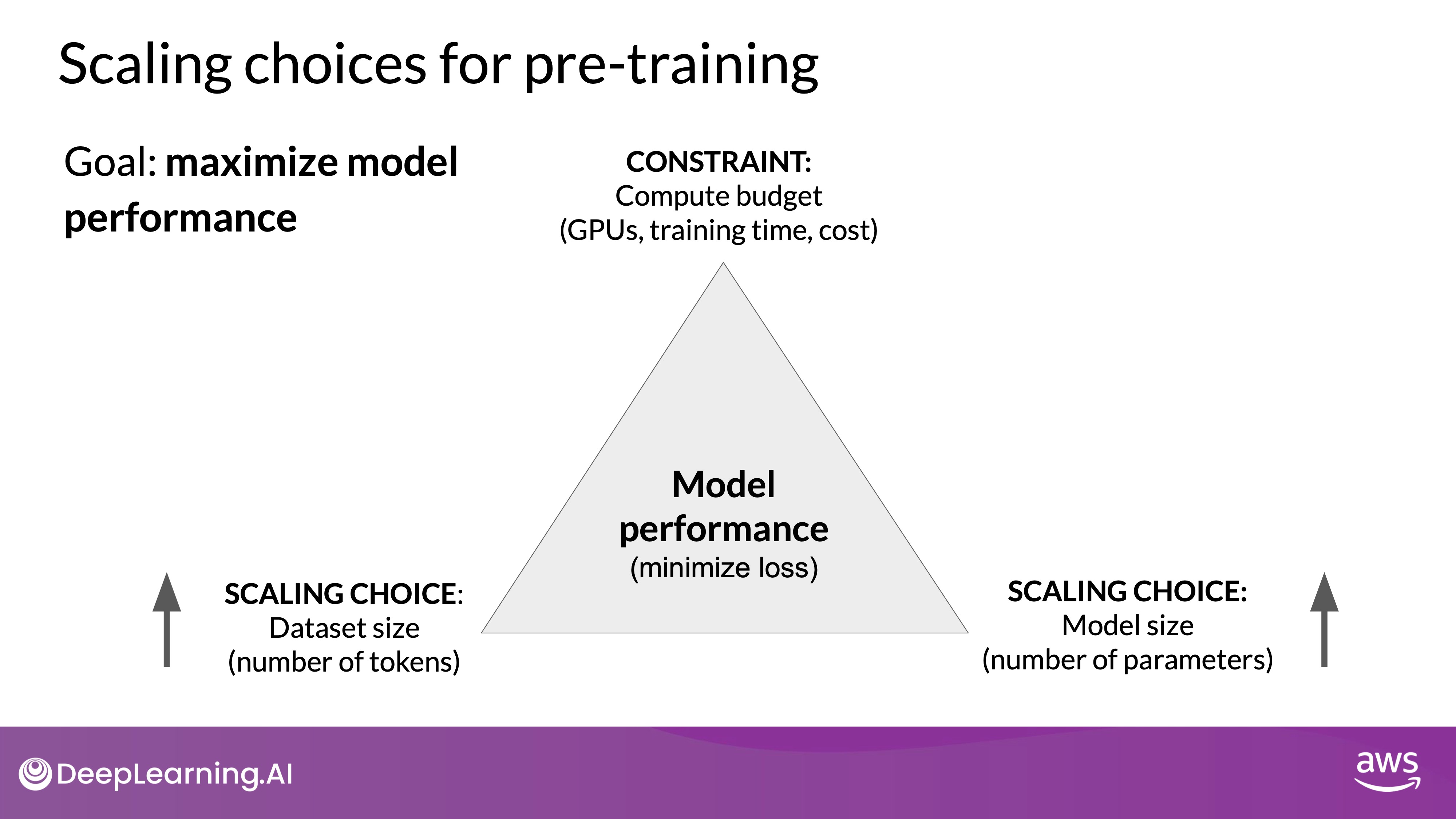
• The Trade-offs in training LLMs:
  • During pre-training, the goal is to maximize a model's performance by minimizing the loss when predicting tokens.
  • To achieve this, you can either increase the size of the dataset or the number of parameters in the model. However, this must be balanced with the compute budget, which includes factors like GPU availability and training time.
• Measurement the compute budget:
  • A common unit of compute is the petaFLOP per second day, which measures the number of floating-point operations performed at a rate of one petaFLOP per second over a day.
  • For example, training with eight NVIDIA V100 GPUs for one day equates to one petaFLOP per second day. More powerful GPUs, like two NVIDIA A100s, can achieve the same compute.
• Comparison of compute requirements for different models:
  • Training larger models requires significantly more compute. For instance, T5 with three billion parameters required around 100 petaFLOP per second days, while GPT-3 with 175 billion parameters needed approximately 3,700 petaFLOP per second days.
  • As models grow in size, they require not only more compute but also more data to perform well.

PetaFlops per second-day

PetaFlops per second-day is a metric used to quantify the computational power required to train large language models (LLMs). It combines the concepts of computational speed and duration, representing the total work done by a system. One petaFLOP stands for one quadrillion (10^15) floating-point operations per second. Thus, a petaFLOP per second-day measures how many floating-point calculations a system can perform in one second, extended over a full 24-hour period.

This metric is crucial for benchmarking, planning, and budgeting the resources needed for training LLMs. For instance, training a model like GPT-3 required approximately 3,700 petaFLOP per second-days, highlighting the immense computational effort involved. By providing a standard measure, this metric helps compare the efficiency and requirements of different training setups and hardware configurations.

If a system runs at 1 petaFLOP (one quadrillion operations per second) for one day (24 hours), the total computational work is:

$$1 \text{ petaFLOP} \times 1 \text{ day} = 1 \text{ petaFLOP per second-day}$$

For a system running at a different rate, say 2 petaFLOPs, for one day:

$$2 \text{ petaFLOPs} \times 1 \text{ day} = 2 \text{ petaFLOP per second-days}$$

Similarly, if a system runs at 1 petaFLOP for half a day:

$$1 \text{ petaFLOP} \times 0.5 \text{ days} = 0.5 \text{ petaFLOP per second-days}$$

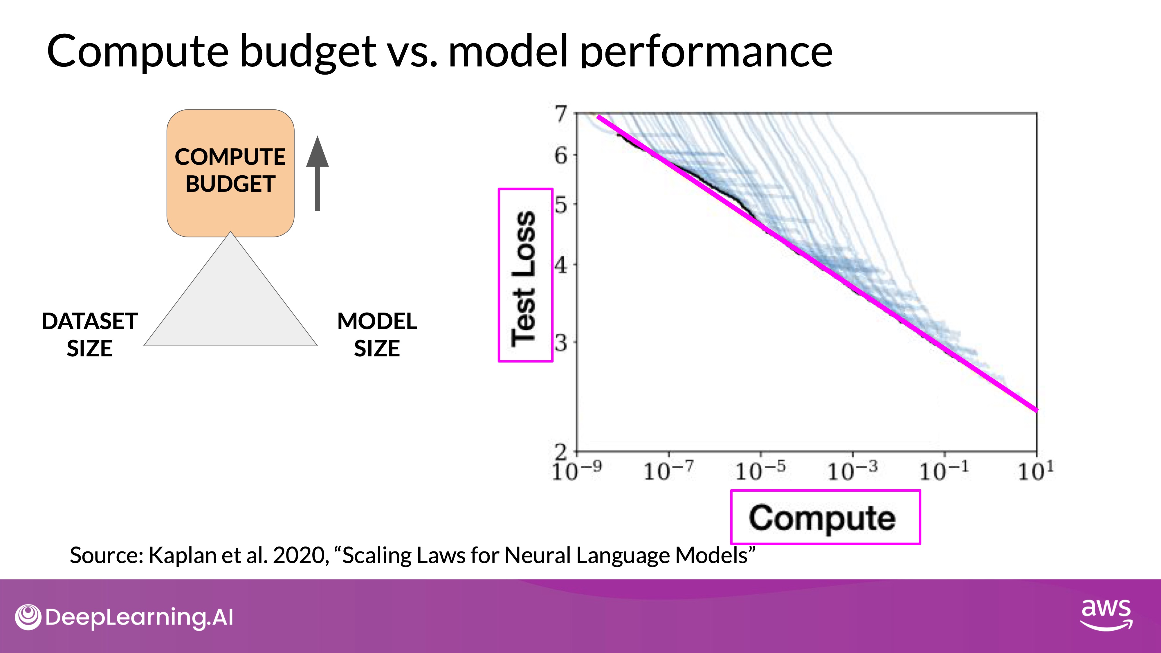
Power-Law Relationships

• Model Performance and Compute Budget:
  • There is a power-law relationship between compute budget and model performance, where performance improves predictably as compute increases.
  • Graphs from OpenAI research show that as the compute budget increases, test loss decreases, suggesting that larger compute budgets generally lead to better-performing models.
  • Source: DeepLearning.AI - Learn the fundamentals of generative AI for real-world applications
• Impact of Training Dataset Size:
  • Holding compute budget and model size constant, increasing the dataset size also improves performance.
  • Similarly, with constant compute budget and dataset size, increasing the model parameters improves performance.

Compute-Optimal Models

Source: DeepLearning.AI - Learn the fundamentals of generative AI for real-world applications

• Chinchilla Paper - the page link:
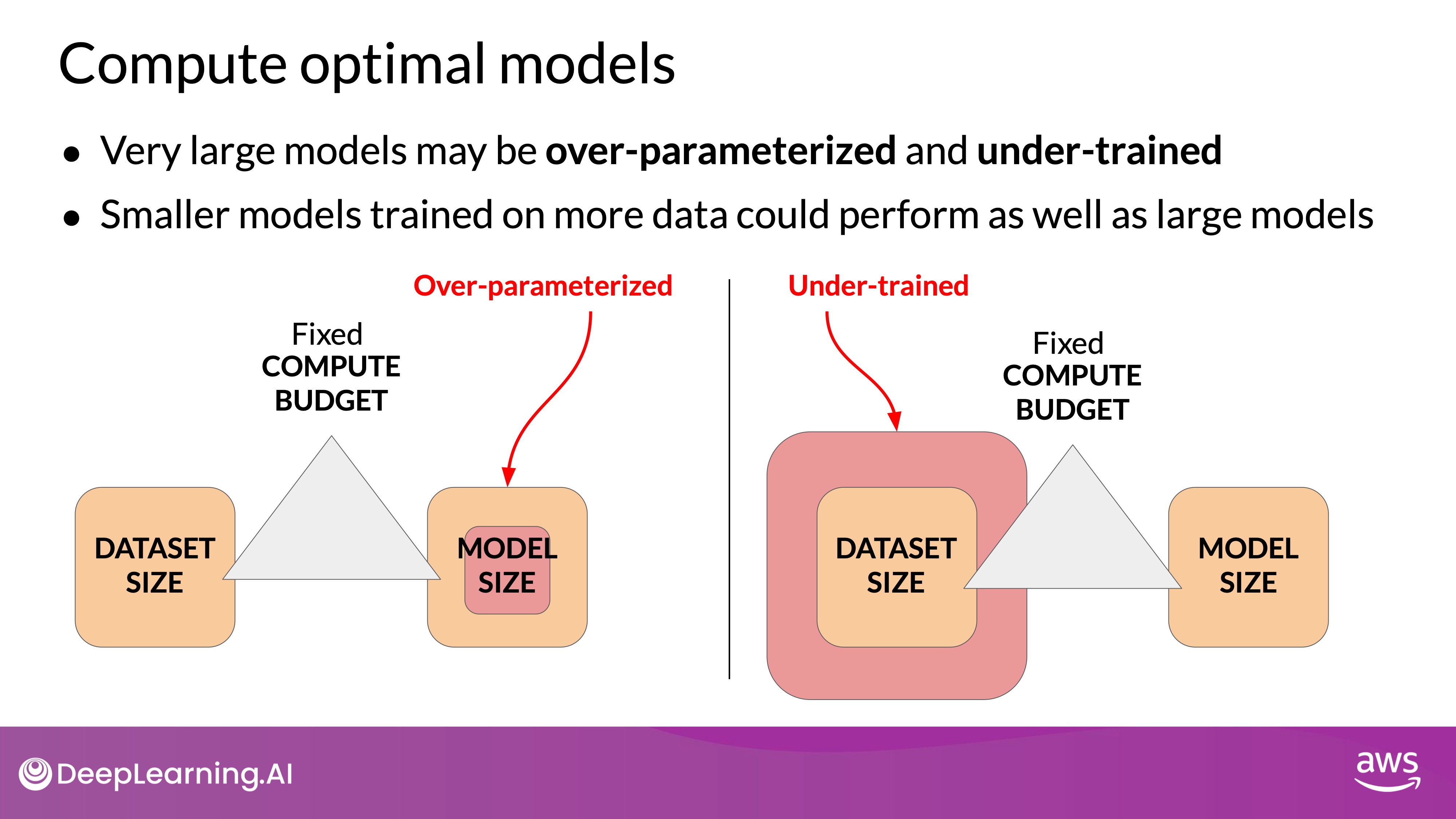
  • Research led by Jordan Hoffmann and others explored the optimal balance of model parameters and training data size for a given compute budget.
  • The study found that many large models like GPT-3 are over-parameterized and under-trained. Smaller models trained on larger datasets can achieve similar or better performance.
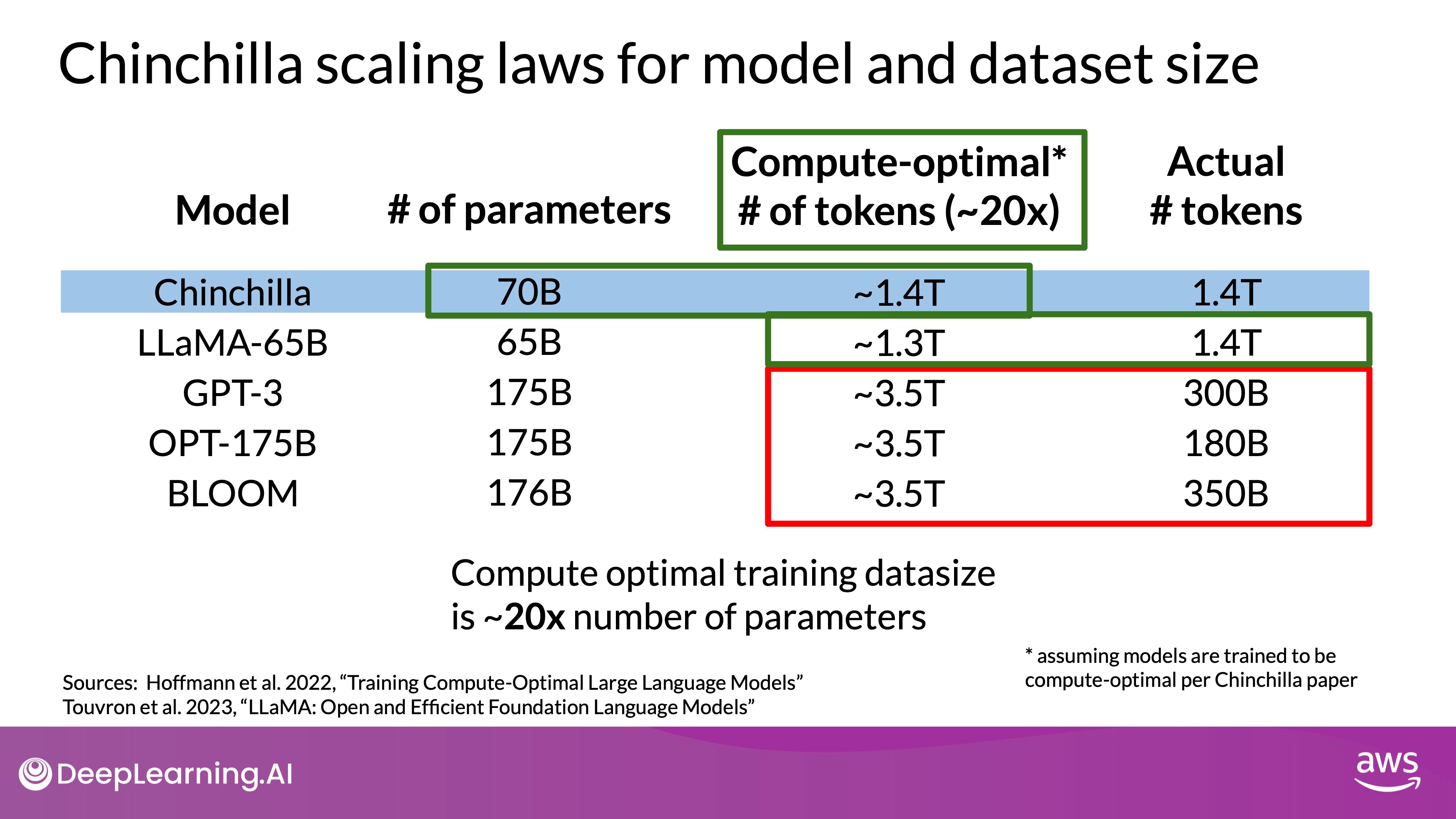
• Key Findings:
  • The optimal training dataset size is about 20 times the number of parameters in the model.
  • For example, a 70 billion parameter model should ideally be trained on 1.4 trillion tokens.
  • Source: DeepLearning.AI - Learn the fundamentals of generative AI for real-world applications
  • Examples:
  • LLaMA, trained on 1.4 trillion tokens, follows this optimal ratio closely.
  • Compute-optimal models like Chinchilla outperform non-optimal models like GPT-3 in various tasks.

Because of the Chinchilla Paperm, the implications for model development is shifting from "bigger is better" to optimizing model size and training data for better performance within a given compute budget. Models like Bloomberg GPT, which follow the compute-optimal guidelines, achieve high performance with fewer parameters.

The Chinchilla Law

The "Chinchilla Law" is a concept from the 2022 paper "Training Compute-Optimal Large Language Models," which identifies the optimal balance between model size, training dataset size, and compute budget for large language models (LLMs). The research suggests that many large models, such as GPT-3, are over-parameterized and under-trained, indicating that they could perform better if trained with larger datasets relative to their size. Specifically, the optimal training dataset should be about 20 times the number of model parameters. This balance ensures that the model fully leverages the data, avoiding inefficiencies associated with having too many parameters but insufficient data.

Why the Pretraining Scaling Laws Are Correct

1. Joint Increase of Dataset Size and Model Size:
   • According to Chinchilla Law, both dataset size and model size must be increased together to prevent bottlenecks. If the dataset size is increased without scaling the model size, the model may not effectively utilize the additional data, leading to suboptimal performance. Conversely, a larger model without sufficient data will not train effectively, underscoring the need for joint scaling.
2. Relationship Between Model Size and Training Tokens:
   • The Chinchilla paper demonstrates a power-law relationship between model size and the optimal number of training tokens. This means that models need an appropriately large dataset relative to their parameters to achieve optimal performance. Many large models are over-parameterized, meaning they have more parameters than needed for the amount of training data, leading to inefficiencies.
3. Compute Budget Measured in PetaFlops per Second-Day:
   • "PetaFlops per second-day" is a metric that effectively captures the compute budget required for training models, reflecting both hardware capability and training duration. This measure helps in understanding the resources needed to train models optimally, aligning with the Chinchilla Law's emphasis on balancing compute budget with model and dataset size for efficient training.

Pre-training for domain adaptation

Challenges

• Using Existing Models vs. Pre-training
  • Existing Models: Generally, using pre-existing large language models (LLMs) can save significant time and expedite the development of your application.
  • Pre-training from Scratch: Necessary when your target domain uses specific vocabulary and language structures not common in everyday language, especially in specialized fields like law, medicine, finance, or science.
• Domain-Specific Language Challenges
  • Because models learn their vocabulary and understanding of language through the original pretraining task. Pretraining your model from scratch will result in better models for highly specialized domains like law, medicine, finance or science.
  • Legal Domain: Terms like "mens rea" and "res judicata" are rarely found outside legal contexts, posing challenges for general LLMs. Legal jargon and redefined everyday terms (e.g., "consideration" in contracts) necessitate domain-specific training for accurate comprehension and usage.
  • Medical Domain: Medical terminology and shorthand used in prescriptions (e.g., "1 tab PO qid ac and hs") are not commonly found in general training datasets, requiring specialized training for accurate interpretation.

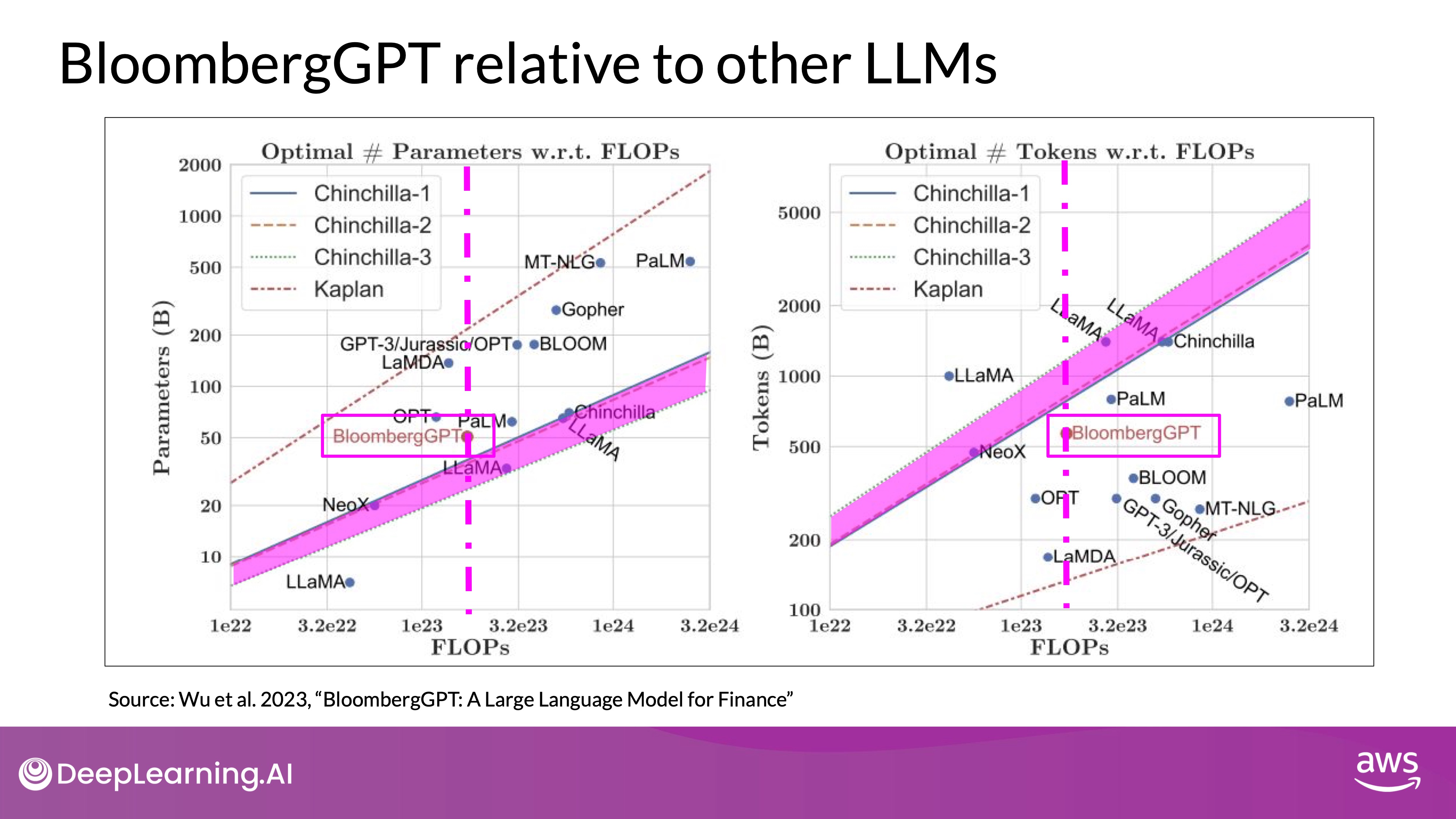
BloombergGPT

BloombergGPT was pre-trained using both financial and general-purpose text data to optimize performance in the finance domain while maintaining general LLM capabilities. The model used 51% financial data and 49% public data to achieve best-in-class results on financial benchmarks and competitive performance on general benchmarks.

Source: DeepLearning.AI - Learn the fundamentals of generative AI for real-world applications

• On the left, the diagonal lines trace the optimal model size in billions of parameters for a range of compute budgets.
  • In terms of model size, you can see that BloombergGPT roughly follows the Chinchilla approach for the given compute budget of 1.3 million GPU hours, or roughly 230,000,000 petaflops. The model is only a little bit above the pink shaded region, suggesting the number of parameters is fairly close to optimal.
• On the right, the lines trace the compute optimal training data set size measured in number of tokens.
  • However, the actual number of tokens used to pretrain BloombergGPT (569 billion tokens) is below the recommended Chinchilla value for the available compute budget. The smaller than optimal training data set is due to the limited availability of financial domain data due to the limited availability of financial data (real world constraints).
• Pink line and region:
  • The dashed pink line on each graph indicates the compute budget that the Bloomberg team had available for training their new model.
  • The pink shaded regions correspond to the compute optimal scaling loss determined in the Chinchilla paper.

Real-World Constraints (Trade-offs)

In practice, constraints like data availability can force trade-offs between ideal model design and achievable training datasets.